Introduction to Neural Networks with Architecture Guide

Artificial Intelligence has transformed the tech landscape, and at the core of this revolution lies Neural Networks. These models mimic the way human brains function, enabling machines to recognise patterns, make decisions, and even learn from mistakes. Whether it's image recognition, natural language processing, or autonomous vehicles—neural networks are the backbone of modern machine learning solutions.

In this blog post, we’ll break down the architecture of neural networks, explore various activation functions, and walk through the processes of forward propagation and backpropagation, enriched with diagrams and code snippets. The article is crafted with a professional touch, suitable for both beginners and developers aiming to enhance their practical skills.

What is a Neural Network?

A Neural Network is a series of algorithms that attempts to recognise relationships in data through a process that mimics how the human brain operates. They consist of layers of nodes (neurons), each connected and responsible for transforming input data to meaningful output.

Keyword usage: Introduction to Neural Networks helps beginners and professionals understand the core of machine learning models with real-world applications.

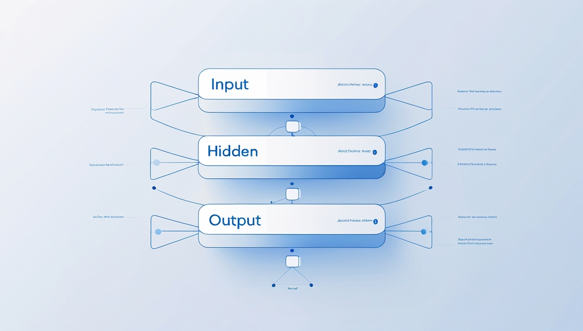
Neural Network Architecture

The architecture of a neural network refers to the arrangement of neurons in layers:

1. Input Layer: Receives the raw data.

2. Hidden Layers: Perform calculations and extract features.

3. Output Layer: Produces the final prediction/output.

Each connection has a weight and bias, which are adjusted during the training process.

Illustration:

Input Layer     Hidden Layer(s)     Output Layer
[ x1, x2, x3 ] → [ h1, h2, h3 ]  →  [ y ]

Each node applies an activation function to the weighted sum of inputs, producing outputs for the next layer.

Activation Functions Explained

Activation functions introduce non-linearity in the network, allowing it to learn complex patterns.

Popular Activation Functions:

Name	Formula	Use Case
Sigmoid	σ(x) = 1 / (1 + e^−x)	Binary classification
ReLU	f(x) = max(0, x)	Most hidden layers
Tanh	f(x) = (e^x − e^−x) / (e^x + e^−x)	Normalised hidden output
Softmax	exp(xi)/Σexp(xj)	Multiclass classification

Visual Example:

import numpy as np
import matplotlib.pyplot as plt

x = np.linspace(-10, 10, 100)
relu = np.maximum(0, x)
sigmoid = 1 / (1 + np.exp(-x))
tanh = np.tanh(x)

plt.plot(x, relu, label='ReLU')
plt.plot(x, sigmoid, label='Sigmoid')
plt.plot(x, tanh, label='Tanh')
plt.title('Activation Functions')
plt.legend()
plt.show()

Forward Propagation: Step-by-Step

In forward propagation, input data flows through the network layer by layer:

1. Multiply inputs by weights.

2. Add bias.

3. Apply activation function.

4. Send the result to the next layer.

This continues until the output layer generates the prediction.

Formula:

For one neuron:
z = w*x + b
a = activation(z)

This process allows the network to generate predictions before calculating error.

Backpropagation: Behind the Learning Process

Backpropagation is how a neural network learns by adjusting its internal parameters based on prediction error.

Process:

1. Compute error using Loss Function.

2. Calculate gradient of loss w.r.t. each weight using chain rule.

3. Update weights using Gradient Descent.

Example with Mean Squared Error (MSE):

loss = (y_pred - y_true)**2
gradient = 2 * (y_pred - y_true) * derivative_of_activation

Then:
weights = weights - learning_rate * gradient

This iterative optimisation leads to improved accuracy over time.

Code Snippet: Build a Neural Network with Python

Here’s a minimal example using TensorFlow:

import tensorflow as tf
from tensorflow.keras.models import Sequential
from tensorflow.keras.layers import Dense

# Sample data
X = [[0,0],[0,1],[1,0],[1,1]]
y = [[0],[1],[1],[0]]  # XOR problem

# Neural Network
model = Sequential()
model.add(Dense(4, input_dim=2, activation='relu'))
model.add(Dense(1, activation='sigmoid'))

model.compile(optimizer='adam', loss='binary_crossentropy', metrics=['accuracy'])
model.fit(X, y, epochs=100, verbose=0)

print("Prediction:", model.predict([[1, 1]]))

This code illustrates a simple 2-layer network using ReLU and Sigmoid, ideal for binary problems like XOR.

Expert Opinion

Dr. Arvind Sharma, AI Researcher at IIT Delhi, says:

"A clear Introduction to Neural Networks is vital for grasping how deep learning works. Understanding architecture and backpropagation lays the groundwork for real-world applications."

Final Thoughts

A solid Introduction to Neural Networks includes understanding its architecture, how activation functions guide signal flow, and the importance of forward and backward propagation in training. Whether you are building from scratch or using libraries like TensorFlow or PyTorch, grasping these fundamentals ensures a confident start in your AI journey.

Learning neural networks is a continuous path—start simple, then explore convolutional networks, recurrent layers, and transformer models. As always, code, train, experiment—and learn.

Disclaimer:
While I am not a certified machine learning engineer or data scientist, I have thoroughly researched this topic using trusted academic sources, official documentation, expert insights, and widely accepted industry practices to compile this guide. This post is intended to support your learning journey by offering helpful explanations and practical examples. However, for high-stakes projects or professional deployment scenarios, consulting experienced ML professionals or domain experts is strongly recommended.
Your suggestions and views on machine learning are welcome—please share them below!

Previous Post 👉 Model Evaluation & Cross-Validation Techniques – Metrics: accuracy, precision, recall, F1 score, AUC

Read more AI tutorials here